At Alinia, a significant part of our research effort goes into building world-class policy models. For most customers, these are used in real time through our API to allow or block chatbot interactions in highly regulated environments, where detecting policy violations quickly is just as critical as detecting them accurately.

Traditionally the so-called Engineering Triangle says: when considering among fast, good, and cheap, you must pick two. As it turns out, when every single chatbot interaction in a financial institution goes through the Alinia API, customers demand all three.

So these constraints are baked into our research and development effort from the very onset: our policy models need to be small so that they can run fast on cheaper hardware, while retaining excellent precision and recall.

In this article we share some useful techniques that combined helped us cut our P95 latency by 28% and increase our throughput by 60%.

We assume the reader is familiar with LLMs, what a GPU is and that it runs parallel programs called kernels, but not necessarily how it does so. Below we introduce some light educational background too, necessary to contextualize the article. Feel free to skip it if you are already familiar with Arithmetic Intensity and compute vs memory-bound kernels.

Background: GPU compute and memory

A little aside here to help contextualize what comes next. GPUs have a lot of what’s commonly called VRAM or GPU memory. They also have specialized matrix multiplication units called Tensor Cores (the name varies across vendors, but NVIDIA calls them this).

Tensor Cores are extremely fast at doing matrix multiplication, while GPU memory is extremely slow to read and write from. This duality brings about a hierarchy of caches, as well as a suite of arcane programming techniques to “keep the Tensor Cores fed”, namely making sure that the fastest compute unit in our hardware never has to be wastefully waiting for slow memory operations to complete.

In practice this is often hard, and sometimes impossible, depending on the nature of the algorithms that we wish to compute on our GPU.

Enter Arithmetic Intensity

A useful way to think about this is Arithmetic Intensity, defined as FLOPs (operations like addition or multiplication) divided by the number of bytes read from or written to memory.

For example, a kernel adding two BF16 vectors together has an Arithmetic Intensity of 1/6, because the whole thing consists of reading each element from both vectors, performing a single addition, and writing a new vector of the same size at the end:

1 addition / (4 bytes read + 2 bytes written)

The “roofline” model: compute-bound vs memory-bound kernels

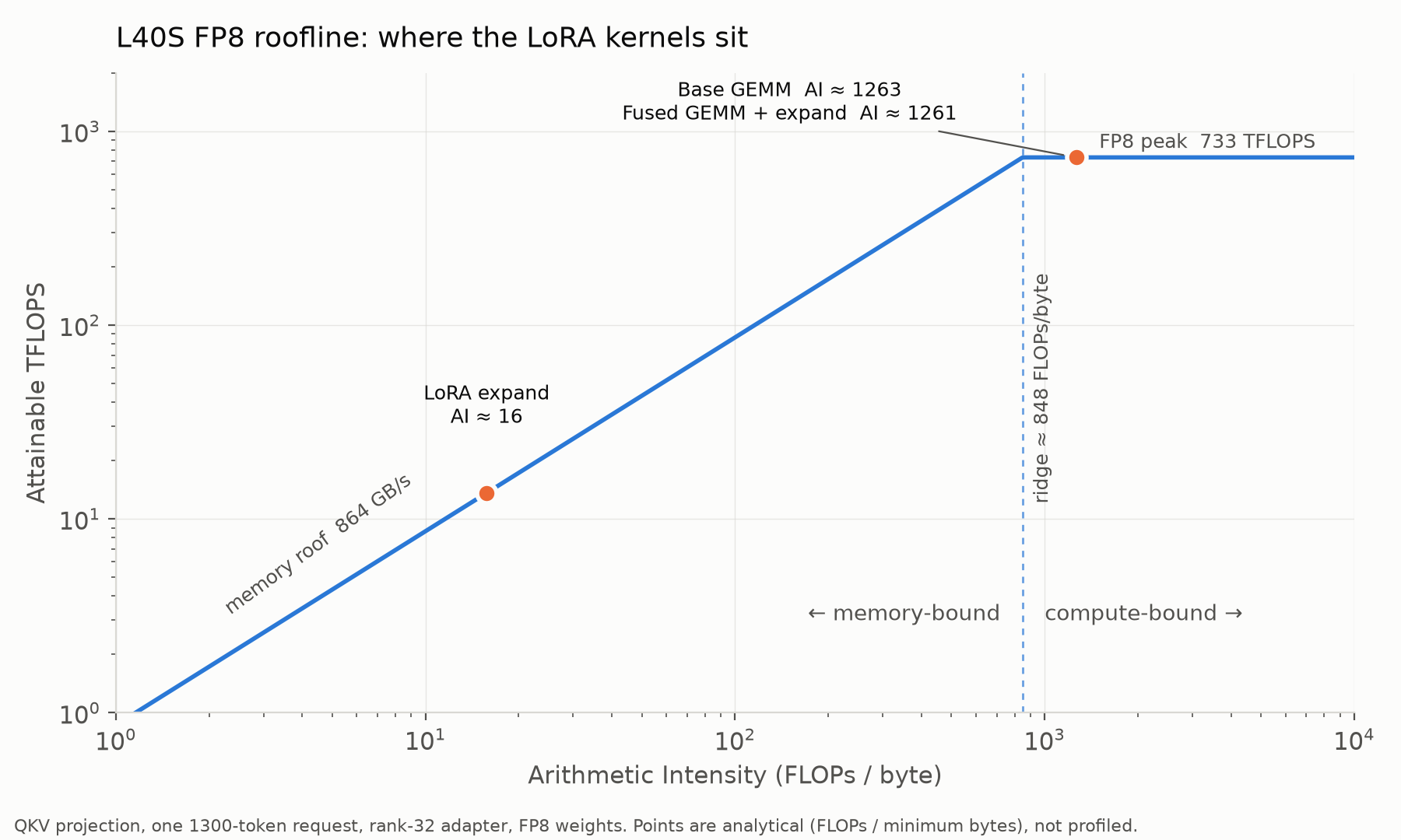
How do we know if an Arithmetic Intensity of 1/6 is good or bad? If our goal is to keep the Tensor Cores fed, we can take the theoretical peak FLOPs / second (called FLOPS with a capital S, confusingly) that they can reach on our particular GPU, and divide it by the peak bandwidth that the GPU memory can provide.

An NVIDIA L40S GPU advertises a peak of 733 TFLOPS when doing matrix multiplication in FP8 precision, and a peak memory bandwidth of 864 GB/s. This gives about 850 FLOPs / byte, which we call our ridge.

If our kernel’s Arithmetic Intensity falls below our ridge, it’s said to be memory-bound, which intuitively means it reads or writes a lot of memory and computes very little, so the Tensor Cores spend most of the time idle waiting for memory operations to complete, which is wasteful.

If it falls on or above the ridge, it’s said to be compute-bound, which means the Tensor Cores are always busy and work arrives faster than they can complete it, which is exactly what you want when paying such a premium for these expensive GPUs.

Now that we have a better grasp on these concepts, let’s look at what our inference setup looks like.

Our particular workload

Architecturally, our policy models are low-rank adapters on top of Seny, our regulatory base model, which is a decoder transformer. The output of a request is a calibrated probability of the provided input being in violation of the policy in question. We serve a lot of those policy models from a single GPU thanks to multi-LoRA inference, that is, serving multiple requests (each one targeting a different low-rank adapter) in the same forward pass.

Typical LLM inference setups consist of two distinct stages: prefill and decode. Prefill processes the entire input in parallel, populating the KV cache and giving us the first output token for free. For any subsequent output tokens you may want to produce, the decode stage uses that cache and the last produced token to produce the next one.

In our case we deviate quite a bit from this traditional recipe. We forgo the decode step entirely, and perform only prefill on the input. We also don’t do any kind of sampling, but instead focus on two distinct tokens in our vocabulary, let’s call them Compliant and Violation, to calculate the calibrated probability of a violation with a softmax over the two logits and Platt calibration.

Prefill-only workloads are nice

The advantage of prefill-only workloads is that they tend to be naturally compute-bound, that is, bottlenecked mostly by the GPU’s Tensor Cores. That is especially true for both large models and large batch sizes, neither of which we can afford to leverage unfortunately, due to our strict latency requirements.

However, even in our regime of small models and small batch sizes, the matrix multiplications still dominate, at about 80% of GPU time of a single request. With larger batches, they do reach higher efficiency due to the cost of reading the model weights being amortized among many requests.

But we can’t just batch requests to our heart’s content, again, because larger batches mean higher latency. So we carefully tune the batch size to maximize throughput while staying under our aggressive latency SLOs.

Hardware

NVIDIA L40S is our GPU of choice. It packs 733 TFLOPS in FP8 (8-bit floating point precision), which powers most of our computations. That is around a third of an H100 SXM’s, while being almost 4x cheaper and more widely available.

How we do inference

Here we discuss the tricks and techniques that helped us get to where we are today, starting from the more common towards the more esoteric and workload-specific.

Quantization

As hinted just earlier, quantization is the first technique we found value in. Our base model weights are quantized ahead of time to FP8, which makes most of our matrix multiplications able to utilize the FP8 Tensor Cores. However, we did not find empirical gains in quantizing the KV cache.

Surprising perhaps? While a traditional LLM workload would very much care about optimizing the KV cache by compressing it or making access to it more efficient, in our case it’s useful only as a cross-request prefix cache, because we don’t do autoregressive decoding. A lot of the GPU memory that would otherwise be dedicated to it is then available to host thousands of warm LoRA adapters. Prefill-only workloads are indeed nice.

Also, by keeping attention and the KV cache in 16 bits, we retain our model’s trained accuracy without leaving latency gains on the table.

Tokenization

We introduced our own tokenization pipeline based around Gigatoken, an excellent open-source, Rust-based tokenizer that helped us shave about 5% off single request latency.

CUDA Graphs

We use CUDA Graphs, which are like execution graphs compiled ahead of time. They help ease pressure on the CPU by reducing kernel launch overhead.

The gains from this intervention were well within noise, but we saw no reason not to use it, seeing kernel launches per call falling from 766 to 42.

Though we have not measured it, it is reasonable to think they may help in more traditional decode-heavy setups.

Fused classification head

During inference, our inputs are tokenized, embedded (projected from token space to latent space) and then go through all the transformer layers.

After that they are still in latent space, which means they are not tokens that we can read as words. We need to project them back to token space, and that is called the unembed, precisely because it’s the opposite of the embedding operation.

Unembedding is a massive matrix multiplication with a hidden_dim x vocab_size matrix, and it produces a logit for each token in our vocabulary, so that traditional autoregressive decoding can convert those logits into probabilities and sample the next token from them.

Our policy models only care about two tokens: our previously introduced Compliant and Violation tokens. So why perform a massive matrix multiplication and produce hundreds of thousands of logits, only to extract the two that we care about?

Instead, we perform two dot products to surgically project the residual stream onto a 2-dimensional token space, which saves us time that would otherwise be spent mostly reading a massive weight matrix from (and writing a lot of logits onto) GPU memory, only to be discarded later.

Thanks to this neat trick, tailored specifically to our workload, we measured about a 6% reduction in GPU time for single-requests.

Fused LoRA GEMM

This one is the most impactful and also the deepest in the weeds, so let’s take it one step at a time.

Let’s consider a LoRA adapter that affects the attention QKV projections. We like to think of the base model’s projection of the input as its base facts, and the LoRA adapter contribution as an adapter-specific opinion. We will be using those intuitive terms to aid in the explanation.

The LoRA operation

Transformer inference is full of linear projections like this one, in which x is the input, and W is some matrix of weights. This would compute the base facts about the input x:

base_facts = x @ W

‍

A low-rank adapter, or LoRA, is a weight matrix just like W, but much smaller. It is deconstructed into two lower-rank matrices called A and B where A @ B has the same shape as W. So to project the input x onto this LoRA, (to compute the adapter-specific opinion) we do:

opinion = x @ A @ B

‍

Remember that matrix multiplication is associative, so `x @ (A @ B) = (x @ A) @ B` . This is important, because there are many ways to compute the same mathematical result, some more efficient than others. Now, we just need to add the base facts and the adapter-specific opinion (scaled, to modulate its influence) together:

qkv_output = base_facts + opinion * opinion_scale

‍

Or the fully expanded way:

qkv_output = x @ W + (x @ A @ B) * opinion_scale

‍

The operations making up this chain have their own names in LoRA inference:

• x @ W is just called a GEMM, which stands for General Matrix Multiply.
• x @ A is called LoRA shrink, because intuitively it takes an input activation of some dimension and shrinks it into a lower-dimensional vector.
• If we call the result of shrinking the vector s, then s @ B (plus scaling it and adding it to the base facts) is called the LoRA expand operation, expanding the shrunken vector back into a higher-dimensional vector, scaling that, and adding it onto the base facts.

The default way of computing LoRA

The LoRA operation, as we’ve seen above, is:

‍

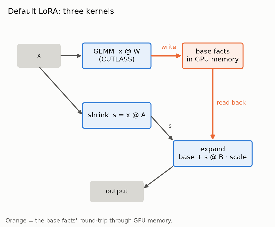
By default, in our specific inference stack, the GEMM will use kernels from CUTLASS, which is NVIDIA’s heavily tuned GEMM library. It is often taken as a ceiling of what one can achieve with custom kernels, so in general it’s a good idea to use it if you can, before bothering to write any code.

Both the base GEMM and shrink are hefty matmuls with good potential for high Arithmetic Intensity. The expand operation is a Triton kernel that ships with SGLang, and it does the s @ B LoRA expand, scales it, and adds it to the base result, in a single fused kernel.

But even doing all these things in a single kernel, expand is still extremely memory bound. There are a couple of factors that contribute to that:

• The only matmul expand does has a tiny inner dimension (it happens to be the low rank dimension of the LoRA). That means fewer Tensor Core operations per output write.
• To add the scaled LoRA opinion onto the base facts, it needs to read the base facts into memory and write the updated version back. For a few hundred token requests and a hidden size of 3072, that can get to half a gigabyte of traffic per forward pass, for a single element-wise addition.

Fusing the base GEMM and LoRA expand

If you view those operations as a graph, both the GEMM and the shrink depend only on the input x. If we reorder the operations and compute s first, we can then fuse the rest in a single kernel:

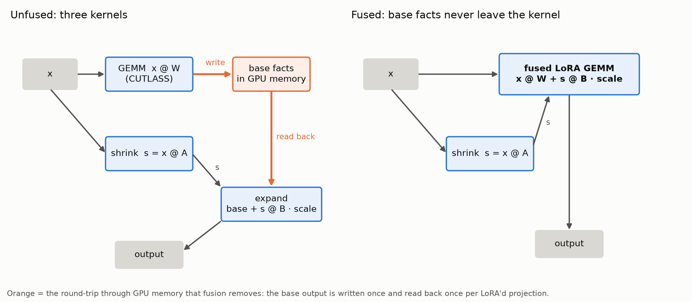
This single fused kernel, by subsuming the very low Arithmetic Intensity expand kernel (about 16 FLOPs/byte) into the base GEMM, ends up saving an expensive round-trip to memory, and it has about the same Arithmetic Intensity as the CUTLASS base GEMM it replaced, keeping us still in the nice compute-bound area:

The first question you should ask yourself when approaching an idea like this is: if you write a custom fused kernel, you’re giving up CUTLASS for the base GEMM. Is it worth it? The only way is to measure with your specific inputs, model and GPU.

In our case, for a single sample request, we saw:

• The original base CUTLASS GEMM took 2.82ms
• SGLang’s stock LoRA expand kernel took 3.10 ms
• Total: 5.92ms

Our custom fused LoRA GEMM kernel took 4.17ms. It is only 1.5x slower than the bare CUTLASS GEMM, despite also doing the expand, which makes it 1.76ms faster end to end.

That may seem modest, but under load, with batching coming into play, we saw our fused kernel bring our P95 latency down as much as 15%, with as much as a 22% increase in throughput for heavy load.

Conclusion

Making Alinia’s policy models fast, good and cheap is undeniably a balancing act, and it’s only achievable when we understand our technical constraints as intimately as the platforms and hardware we depend on. And even with the necessary theoretical understanding, measuring is the only way to know.

We hope you learned something from this article. And if you enjoy this kind of work, we would love to hear from you!